Setup

This tutorial introduces an overview of the Obz library which allows you to connect to the computer vision AI model. It provides a family of feature extraction and explanation methods.

For the simplicity, we provide a pre-trained model and use an existing medical image dataset.

We will go through the scenario step by step. Firstly, let’s start with doing some imports.

import sys
import os
from torch.utils.data import DataLoader
from torchvision.transforms import v2
import torch
from torch import nn
import numpy as np
import gdown
import os
import matplotlib.pyplot as plt

# Repository root directory
repo_root = os.path.abspath(os.path.join(os.getcwd(), ".."))
sys.path.append(repo_root)
#print(repo_root)

Load a pre-trained model

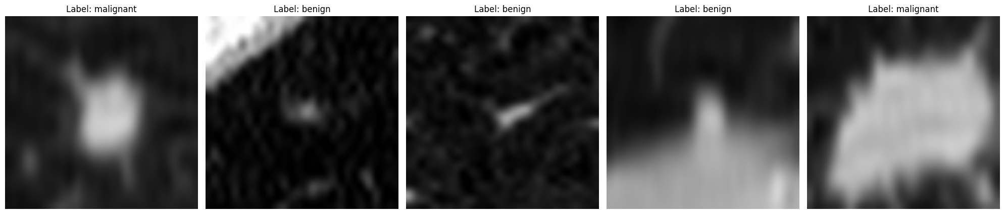
Before you can monitor or visualize the workings of your model using our library, you first need to define the model you want to track.

In this tutorial, we will use a Vision Transformer (ViT) model that has been previously trained and fine-tuned on lung nodules (LIDC) — meaning, the model has already learned to recognize patterns in medical images of lung nodules using a technique called self-supervised learning, specifically with the DINO backbone.

def download_weights(url, output_dir, filename):
    """
    Downloads weights from the given URL if they are not already downloaded.
    """
    os.makedirs(output_dir, exist_ok=True)
    output_path = os.path.join(output_dir, filename)
    
    if not os.path.exists(output_path):
        print(f"Downloading weights to {output_path}...")
        gdown.download(url, output_path)
    else:
        print(f"Weights already exist at {output_path}. Skipping download.")

url = "https://drive.google.com/uc?id=1xUevCbvII5yXDxVxb7bR65CPmgz2sGQA"
output_dir = "tuned_models"
filename = "lidc_dino_s8.pth"
download_weights(url, output_dir, filename)

Weights already exist at tuned_models/lidc_dino_s8.pth. Skipping download.

Configure the ViT classifer based on DINO backbone

We are adding a binary classification head (see how torch.nn.Linear) onto a DINO backbone.

from transformers import ViTConfig, ViTModel

class DINO(nn.Module):
    """
    DINO Transformer model based on Huggingface implementation.
    """
    def __init__(self):
        super().__init__()
        # Backbone
        config = ViTConfig.from_pretrained('facebook/dino-vits8', attn_implementation="eager") # We propose eager implementation to return att scores gracefully.
        self.backbone = ViTModel(config)
        # Classfication head
        self.head = torch.nn.Linear(384, 1)
    
    def forward(self, x: torch.Tensor, output_attentions:bool=False):
        out = self.backbone(x, output_attentions=output_attentions)
        x = out["pooler_output"]
        x = self.head(x)
        if output_attentions:
            att = out["attentions"]
            return x, att
        else:
            return x

We load the pre-trained weights onto this model.

DEVICE = "cuda" if torch.cuda.is_available() else "cpu"
WEIGHTS_PATH = "./tuned_models/lidc_dino_s8.pth"

MODEL = DINO()
MODEL.load_state_dict(torch.load(WEIGHTS_PATH, weights_only=True, map_location=torch.device(DEVICE)))
MODEL = MODEL.to(DEVICE).eval()

Next, let’s prepare the datasets. In general, you will need two separate sets of images:

Reference Dataset: This dataset will be used to extract reference image features and to fit the outlier detection models. In ML, this may be a training dataset.

Inference Dataset: This dataset will be treated as incoming new data on which you want to perform outlier detection. In ML, this may be testing or validation dataset or any new samples in production.

For the tutorial case we will use LIDC-IDRI subset called: Nodule MNIST. This dataset is readily available via MedMNIST package.

# pip install medmnist
from medmnist import NoduleMNIST3D
# Transforms
def take_middle_slice(inpt: np.ndarray):
    """
    NoduleMNIST 3D contains whole nodule volumes, however for this tutorial
    we will utilize only central slice of each example.
    We repeat this slice 3 times, as model expects input to have 3 channels.
    """
    inpt = inpt.squeeze()
    X, Y, Z = inpt.shape
    slice_ = inpt[:, :, Z//2]
    slice_ = torch.Tensor(slice_).unsqueeze(dim=0).repeat(3,1,1)
    return slice_

TRANSFORMS = v2.Compose([v2.Lambda(take_middle_slice),
                         v2.Resize(size=(224,224))
                         ])

NORMALIZE = v2.Normalize(mean=[0.485, 0.456, 0.406], std=[0.229, 0.224, 0.225])

# Datasets
data_dir = "./example_data"
os.makedirs(data_dir, exist_ok=True)

## Reference data. We will use it as source of reference statistics and to "train" OutlierDetector.
ref_set = NoduleMNIST3D(root=data_dir, split="val", size=64, transform=TRANSFORMS, download=True)
## Inference data. We will use it as exemplary source of production data. 
inf_set = NoduleMNIST3D(root=data_dir, split="test", size=64, transform=TRANSFORMS)

# DataLoaders
ref_loader = DataLoader(ref_set, batch_size=32, shuffle=False)
inf_loader = DataLoader(inf_set, batch_size=6, shuffle=True)

## NOTE that for homework, download a training set and train ViT models
# train_set = NoduleMNIST3D(root=data_dir, split="train", size=64, transform=TRANSFORMS, download=True)
# train_loader = DataLoader(train_set, batch_size=32, shuffle=False)

# Labels mapping
CLASS_NAMES = ["benign", "malignant"]

LOGIT2NAME = {
    0: "benign",
    1: "malignant",
}

Visualize the first 5 samples from ref_loader

samples, labels = next(iter(ref_loader))

fig, axes = plt.subplots(1, 5, figsize=(20, 5))
for i in range(5):
    image = samples[i].permute(1, 2, 0).numpy()  # Convert tensor to numpy array and rearrange dimensions
    axes[i].imshow(image, cmap='gray')
    axes[i].set_title(f"Label: {CLASS_NAMES[labels[i].item()]}")
    axes[i].axis('off')

plt.tight_layout()
plt.show()

Data Inspector

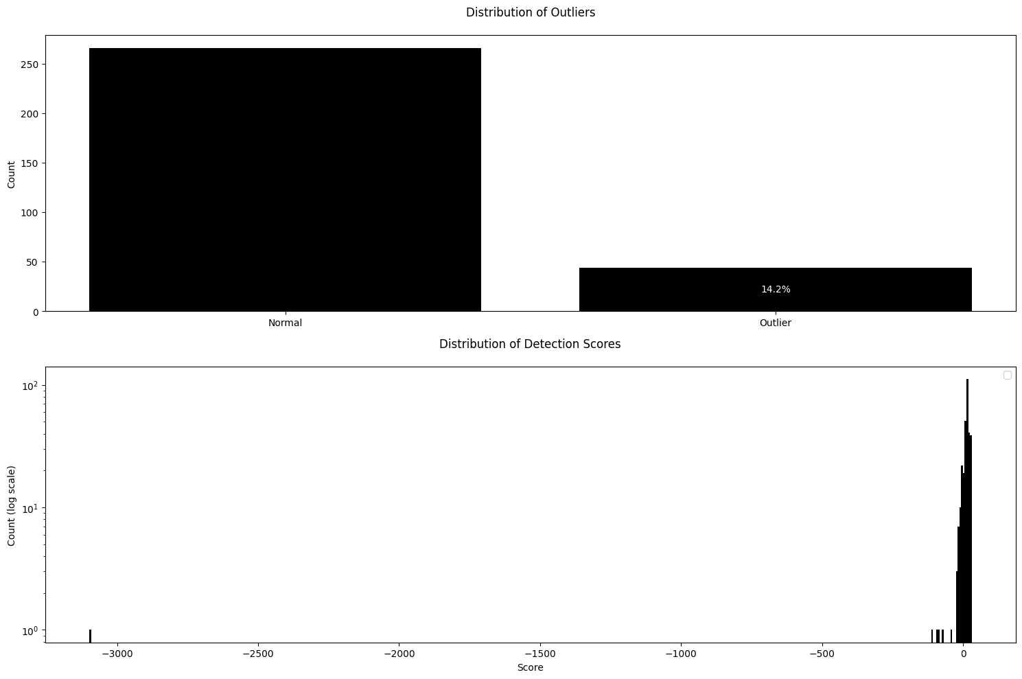
You are now ready to create an Outlier Detector — using the Reference dataset to obtain the typical distribution of visual features and applying that fitted model to the Inference dataset.

The Obz AI package is designed to be highly modular and customizable. As a first step, we’ll import the specific feature extractors and the outlier detection algorithm you want to use.

# Setup OutlierDetector
from obzai.data_inspector.extractor import FirstOrderExtractor, CLIPExtractor
from obzai.data_inspector.detector import GMMDetector, PCAReconstructionLossDetector

Extract First Order Features and build a GMM Detector

FirstOrderExtractor is a straightforward and fast tool designed to extract first-order statistical features from images. These features summarize general properties of the pixel intensity values, such as mean, variance, skewness, etc. For example, they are useful for identifying images that are overly bright/dark or excessively variable in their intensities compared to the Reference dataset.

Note: First-order statistical features are invariant to the arrangement of pixels; in other words, they do not capture spatial relationships within the image.

At any point, you can view the list of features that FirstOrderExtractor computes by accessing its .feature_names attribute. This helps you to understand exactly which statistics are being extracted from your images.

first_order_extrc = FirstOrderExtractor()
first_order_extrc.feature_names

[‘entropy’, ‘min’, ‘max’, ‘10th_percentile’, ‘90th_percentile’, ‘mean’, ‘median’, ‘interquartile_range’, ‘range’, ‘mean_absolute_deviation’, ‘robust_mean_absolute_deviation’, ‘root_mean_square’, ‘skewness’, ‘kurtosis’, ‘variance’, ‘uniformity’]

GMMDetector is an outlier detection method that utilizes a Gaussian Mixture Model (GMM). To configure and use the GMMDetector, please follow the steps below:

  • extractors - Sequence of Extractor objects which process your data. Currently, only the FirstOrderExtractor is accepted.
  • n_components - A number of Gaussian components for the mixture model. This controls the complexity of the model and how finely it can separate data clusters.
  • outlier_quantile - Set the quantile threshold to determine what is considered an outlier. Data points falling below this quantile are classified as outliers.
  • show_progress - If set to True, a progress bar will be displayed during feature extraction to visualize operation progress.

After initialization, you can fit the model to your reference data by calling .fit method with a reference data. Ensure that the data you want to model comes in the form of a PyTorch DataLoader object.

gmm_detector = GMMDetector(extractors=[first_order_extrc], n_components=3, outlier_quantile=0.01, show_progress=True)
gmm_detector.fit(ref_loader)

Your GMM based Outlier Detector is ready to use.

You can pass batches of images in the inference data into .detect() method. This method returns a named tuple with:

  • img_features - extracted features for each image in the batch.
  • outliers - boolean vector indicating if samples in the batch are outliers.

We can run this outlier detection on a single batch of images, and display the outputs.

# Example code to run inference on a single batch
image_batch, _ = next(iter(inf_loader))
detection_results = gmm_detector.detect(image_batch)

# print("Outlier detection results for a batch:")
# print(detection_results.outliers)

# print("First Order Features for a batch:")
# print(detection_results.img_features)

# print("Detection scores:")
# print(detection_results.scores)

Let’s run it on all 310 samples in NoduleMNIST.

## Example code to run inference on multiple batches (upto 1000 samples)
# Process multiple batches from the inference loader
firstorder_total_samples = 0
firstorder_total_outliers = 0
firstorder_outliers = []
firstorder_features = []
firstorder_scores = []

for batch_images, _ in inf_loader:
    # Process batch
    batch_results = gmm_detector.detect(batch_images)
    firstorder_total_outliers += batch_results.outliers.sum()
    firstorder_total_samples += len(batch_results.outliers)

    firstorder_outliers.append(batch_results.outliers.flatten())
    firstorder_features.append(batch_results.img_features['FirstOrderExtractor'].T)
    firstorder_scores.append(batch_results.scores.flatten())

print(f"Processed {firstorder_total_samples} samples")
print(f"Found {firstorder_total_outliers} first-order outliers ({(firstorder_total_outliers/firstorder_total_samples)*100:.2f}%)")

We can visualize the results by creating a histogram of outlier status and a distribution of scores based on GMM. In the second figure, we are plotting the distributrion of scores with y-axis in a log scale.

# Convert lists to numpy arrays for easier manipulation
firstorder_outliers_array = np.concatenate(firstorder_outliers)
firstorder_scores_array = np.concatenate(firstorder_scores)

# Calculate counts for normal and outlier samples
firstorder_outlier_counts = np.bincount(firstorder_outliers_array.astype(int))

# Create the same plots with a minimal look
fig, (ax1, ax2) = plt.subplots(2, 1, figsize=(15, 10))

# Plot 1: Outlier Status Histogram with minimal style
ax1.bar(['Normal', 'Outlier'], firstorder_outlier_counts, color='black')
ax1.set_title('Distribution of Outliers', pad=20)
ax1.set_ylabel('Count')
percentage = (firstorder_outlier_counts[1] / len(firstorder_outliers_array)) * 100
ax1.text(1, firstorder_outlier_counts[1]/2, f'{percentage:.1f}%', ha='center', va='center', color='white')

# Plot 2: Detection Scores Distribution with minimal style
ax2.hist(firstorder_scores_array, bins=500, color='black', edgecolor='none')
ax2.set_yscale('log')  # Set y-axis to logarithmic scale
ax2.set_title('Distribution of Detection Scores', pad=20)
ax2.set_xlabel('Score')
ax2.set_ylabel('Count (log scale)')
ax2.legend()

plt.tight_layout()
plt.show()

XAI Module

XAI Module have components to both provide you with easy-to-use explainability tools and evaluation tools. Module consist of two major ingredients:

  • XAITool - Particular implementations of explainability methods.
  • XAIEval - Evaluation methods for achieved explainability maps.

Let’s do some imports:

from obzai.xai.eval_tool import Fidelity, Compactness
import matplotlib.pyplot as plt
from obzai.xai.xai_tool import CDAM, SaliencyMap, AttentionMap
from obzai.xai.xai_regions import XAIRegions

Predict the cancer status

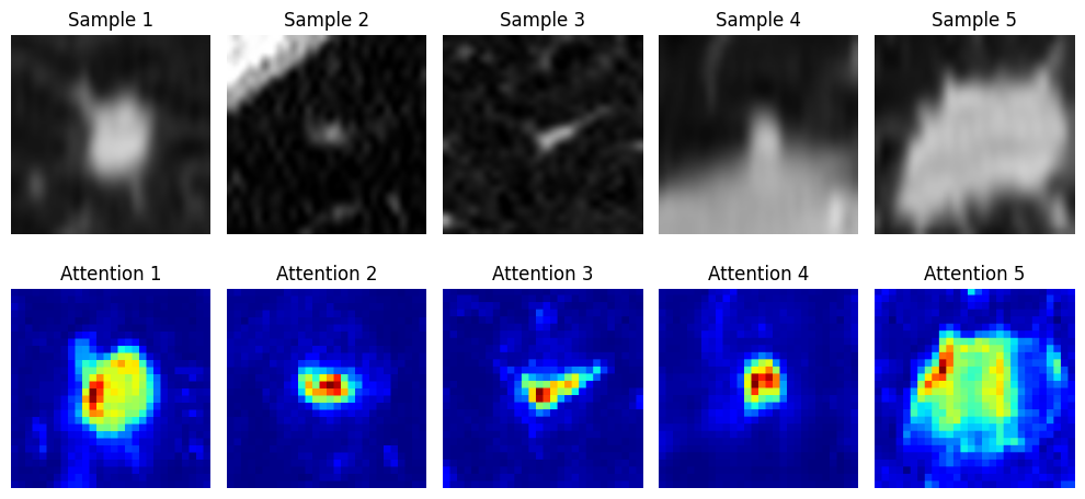
Make the prediction for those 5 samples using the aforementioned MODEL

# Move samples to the appropriate device
samples = samples[:5].to(DEVICE)
labels = labels[:5].to(DEVICE)

# Normalize the samples
#samples = NORMALIZE(samples)

# Perform inference using the model
with torch.no_grad():
    logits = MODEL(samples) 
    predictions = torch.sigmoid(logits).round().squeeze().cpu().numpy()

# Map predictions to class names
predicted_classes = [LOGIT2NAME[int(pred)] for pred in predictions]

# Print the results
for i, pred_class in enumerate(predicted_classes):
    print(f"Prediction for Sample {i + 1}: {pred_class}")

Setup XAITool and XAIEval

Computing importance scores with XAITool
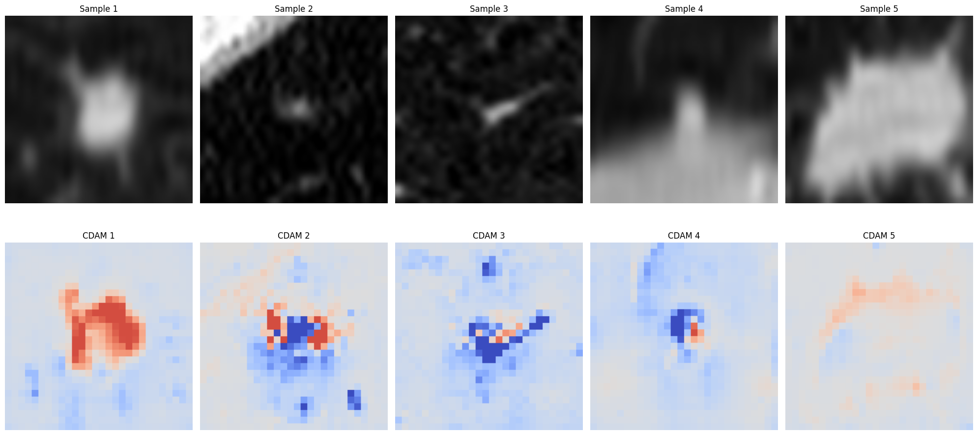
  • cdam_tool - It is an excellent explainability method, highly discriminative with regards to the target class.
  • smooth_grad_tool - Classical and simple XAI method.
  • attention_tool - Classical way to inspect ViT like models.

Choose and set up appropriate XAI tools.

# Choose desired XAI Tools
cdam_tool = CDAM(model=MODEL, 
                 mode='vanilla',                      # CDAM mode
                 gradient_type="from_logits",  # Whether backpropagate gradients from logits or probabilities.
                 gradient_reduction="average",        # Gradient reduction method.
                 activation_type="sigmoid")           # Activation function applied on logits. (Needed when gradients are backpropagated from probabilities.)
# In CDAM you need to specify on which layer you want to create hooks.
cdam_tool.create_hooks(layer_name="backbone.encoder.layer.11.layernorm_before")

attention_tool = AttentionMap(model=MODEL,
                              attention_layer_id = -1,# ID of an attention layer from which to extract attention weights
                              head = None             # ID of attention head to choose. If None, attention scores are averaged.
                              )

Your explainability and evaluation tools are ready to use! Run the XAI method to our data.

# Apply attention_tool on the first ten samples
attention_maps = attention_tool.explain(samples)  # Use the appropriate method to generate attention maps
# Visualize samples and attention maps
fig, axes = plt.subplots(2, 5, figsize=(10, 5))

# First row: Original samples
for i in range(5):
    original_image = samples[i].permute(1, 2, 0).cpu().numpy()  # Convert tensor to numpy array and rearrange dimensions
    axes[0, i].imshow(original_image, cmap='gray')
    axes[0, i].set_title(f"Sample {i + 1}")
    axes[0, i].axis('off')

# Second row: Attention maps
for i in range(5):
    attention_map = attention_maps[i].cpu().numpy()
    axes[1, i].imshow(attention_map, cmap='jet')
    axes[1, i].set_title(f"Attention {i + 1}")
    axes[1, i].axis('off')

plt.tight_layout()
plt.show()

# Visualize attention maps overlaid on samples
fig, axes = plt.subplots(1, 5, figsize=(20, 5))

for i in range(5):
    original_image = samples[i].permute(1, 2, 0).cpu().numpy()  # Convert tensor to numpy array and rearrange dimensions
    attention_map = attention_maps[i].cpu().numpy()  # Convert attention map to numpy array

    # Overlay attention map on the original image
    axes[i].imshow(original_image, cmap='gray')
    axes[i].imshow(attention_map, cmap='jet', alpha=0.5)  # Use alpha for transparency
    axes[i].set_title(f"Sample {i + 1}")
    axes[i].axis('off')

plt.tight_layout()
plt.show()

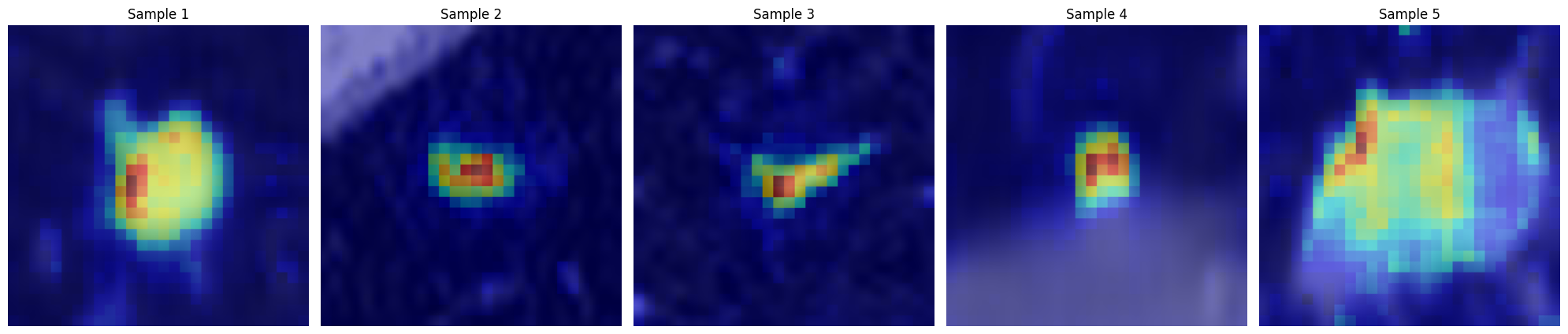
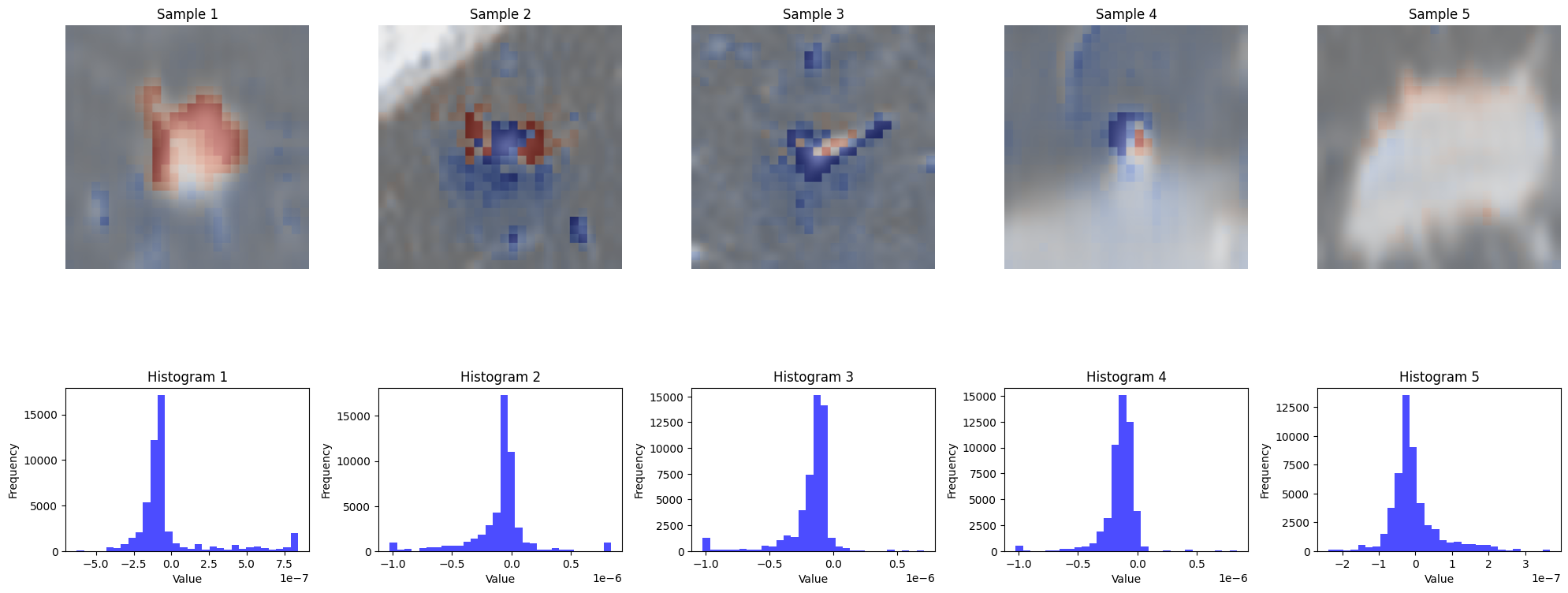
Generate and visualize CDAM maps

# Generate CDAM maps
cdam_maps = cdam_tool.explain(samples, target_idx=[0,0,0,0,0])  # Use the appropriate method to generate CDAM maps
# Visualize samples and CDAM maps
fig, axes = plt.subplots(2, 5, figsize=(20, 10))

# First row: Original samples
for i in range(5):
    original_image = samples[i].permute(1, 2, 0).cpu().numpy()  # Convert tensor to numpy array and rearrange dimensions
    axes[0, i].imshow(original_image, cmap='gray')
    axes[0, i].set_title(f"Sample {i + 1}")
    axes[0, i].axis('off')

# Second row: CDAM maps
for i in range(5):
    cdam_map = cdam_maps[i].squeeze().cpu().numpy()  # Convert CDAM map to numpy array
    axes[1, i].imshow(cdam_map, cmap='coolwarm', vmin=-cdam_maps.abs().max(), vmax=cdam_maps.abs().max())  # Diverging colormap
    axes[1, i].set_title(f"CDAM {i + 1}")
    axes[1, i].axis('off')

plt.tight_layout()
plt.show()

# Visualize CDAM maps overlaid on samples with histogram and color bar
fig, axes = plt.subplots(2, 5, figsize=(20, 10), gridspec_kw={'height_ratios': [4, 1]})

# First row: Original samples with overlaid CDAM maps
for i in range(5):
    original_image = samples[i].permute(1, 2, 0).cpu().numpy()  # Convert tensor to numpy array and rearrange dimensions
    cdam_map = cdam_maps[i].squeeze().cpu().numpy()  # Convert CDAM map to numpy array

    # Overlay CDAM map on the original image
    im = axes[0, i].imshow(original_image, cmap='gray')
    im = axes[0, i].imshow(cdam_map, cmap='coolwarm', alpha=0.5, vmin=-cdam_maps.abs().max(), vmax=cdam_maps.abs().max())  # Use alpha for transparency
    axes[0, i].set_title(f"Sample {i + 1}")
    axes[0, i].axis('off')

# Second row: Histogram of CDAM map values
for i in range(5):
    cdam_map = cdam_maps[i].squeeze().cpu().numpy()  # Convert CDAM map to numpy array
    axes[1, i].hist(cdam_map.ravel(), bins=30, color='blue', alpha=0.7)
    axes[1, i].set_title(f"Histogram {i + 1}")
    axes[1, i].set_xlabel('Value')
    axes[1, i].set_ylabel('Frequency')

plt.tight_layout()
plt.show()

Evaluating XAI methods with XAIEval

There are several Explainable AI (XAI) methods available, each with their own advantages and limitations. Obz AI offers a set of evaluation tools to help assess the quality of XAI methods.

fidelity_tool measures how accurately a given XAI method reflects the model’s true decision process. It does this by systematically perturbing input features based on their importance scores and observing the resulting change in the model performance.

compactness_tool evaluates how sparse and concentrated the importance scores are. A more compact set of importance scores is often easier for humans to interpret, as it highlights the most relevant features in a concise manner.

By using these tools, you can better understand and compare the effectiveness and interpretability of different XAI approaches.

First, instantiate both evaluation methods:

# XAIEval:
fidelity_tool = Fidelity(model=MODEL, device=DEVICE) # Needs to specify the device
compactness_tool = Compactness()
# Evaluating the XAI method
scores_fid = fidelity_tool.score(samples, cdam_maps, target_logits=[0,0,0,0,0])  # Use the appropriate method to score fidelity
scores_comp = compactness_tool.score(cdam_maps)
print("Fidelity: ", scores_fid)
print("Compactness: ", scores_comp)

In general, we would average each of fidelity and compactness scores over all samples to obtain an overall score. An overall score helps us to understand if the XAI method applied on this particular model and dataset is accurate or compact.

High fidelity scores indicate more accurate XAI methods according to perturbation-based accuracy curves. See Brocki and Chung (2023) for further details.

High compactness score is considered better as a more compact set of importance scores is often easier for humans to interpret. Such a XAI map highlights the most relevant features in a concise manner.